How to Predict Migration Patterns using Auspost Movers Statistics Data and Snowflake’s Cortex ML functions

How to Predict Migration Patterns using Auspost Movers Statistics Data and Snowflake’s Cortex ML functions

Data consultancy, Data Army taps into the hidden insights of the Australia Post Movers Statistics dataset to forecast the future hotspots in Australia—predicting where people are likely to move next.

By analysing trends in mail redirection requests through the Time Series Forecasting function, we provide valuable insights with precision.

This advanced analysis is a feature of Snowflake Cortex, Snowflake’s comprehensive Artificial Intelligence and Machine Learning service, designed to empower your decisions with data-driven intelligence.

Overview of Data Used

  • The primary dataset is the Australian Movers Statistics currently available from The Proptech Cloud with a limited free trial. Updated monthly, it contains de-identified and aggregated data on moves across Australia based on mail redirection requests for the previous 5 years. For this exercise, we used the data from February 2019 to January 2024. Each entry in the data includes the postcode the household relocated from, the postcode the household relocated to, the month of relocation and the number of the people that relocated.
  • The secondary dataset used is the Geography Boundaries & Insights – Australia, specifically Australian Bureau of Statistics (ABS) 2021 Postcode Boundary Data (ABS_POA_2021_AUST_GDA2020) to conduct geospatial visualisations. This dataset is free from The Proptech Cloud.

Australia Post Movers Statistics Data

This dataset contains five years of de-identified, aggregated information on past moves captured by Australia Post’s Mail Redirection service.

Access Australia Post mail redirect statistics now to help you develop competitive data-driven strategies.

Introduction to Snowflake Functionality & Technology Stack

  • The Snowflake Forecasting Model is part of the Snowflake Cortex ML- Powered Functions. This model uses a Machine Learning algorithm to predict future trends from historical data.
  • SnowPark which is the set of libraries in Snowflake which will allow us to deploy and process the data pipeline using Python
  • Streamlit which is used to visualise the forecasts created using interactive Python apps. This functionality is fully integrated within the Snowflake Platform

Introduction to Snowflake’s Forecasting Model

Snowflake Cortex is a service by Snowflake which offers Machine Learning (ML) and Artificial Intelligence (AI) solutions.

This blog will focus on using the Time-Series Forecasting Model which is part of this service. The ML forecasting model used in this algorithm is Gradient Boosting (GB).

The intuition behind the GB algorithm is that the combination of multiple models that learn and improve on each other will perform better than one model. To implement this approach, the GB algorithm will firstly implement the best possible model on the dataset.

The second model will assess where the first model performs poorly and try to improve on these areas. This process continues and the models continue to learn and iterate on one another until the model iteration process no longer improves the model outcomes and therefore the optimal model combination is found and used for predictions.

The GB algorithm is very popular due to its ability to learn from itself and it performs very strongly in many different ML problems. One of the typical challenges in using the GB model is that it is usually very computationally expensive and time consuming to iterate and find the optimal model. The advantage of using the Snowflake Cortex Machine Learning Powered Forecasting Model is that it is extremely quick to compute on even very large datasets as it leverages Snowflake’s existing highly scalable infrastructure.

Technical How-To Guide

The forecasting model example shown will use Snowpark to create the data pipeline and use Streamlit for the data visualisations.

Step 1: Accessing the data

  1. Go to the link on the listing to access the Australia Post – Movers Statistics Data.
  2. Click the “Access Data Listing on Snowflake Marketplace” button to access the data listing on the Snowflake Marketplace
  3. Click the ‘Get’ button and the top right of the page to access the Australian Post Movers Statistics Account. This will then redirect to a link to either create a new Snowflake account or sign in if one already exists.
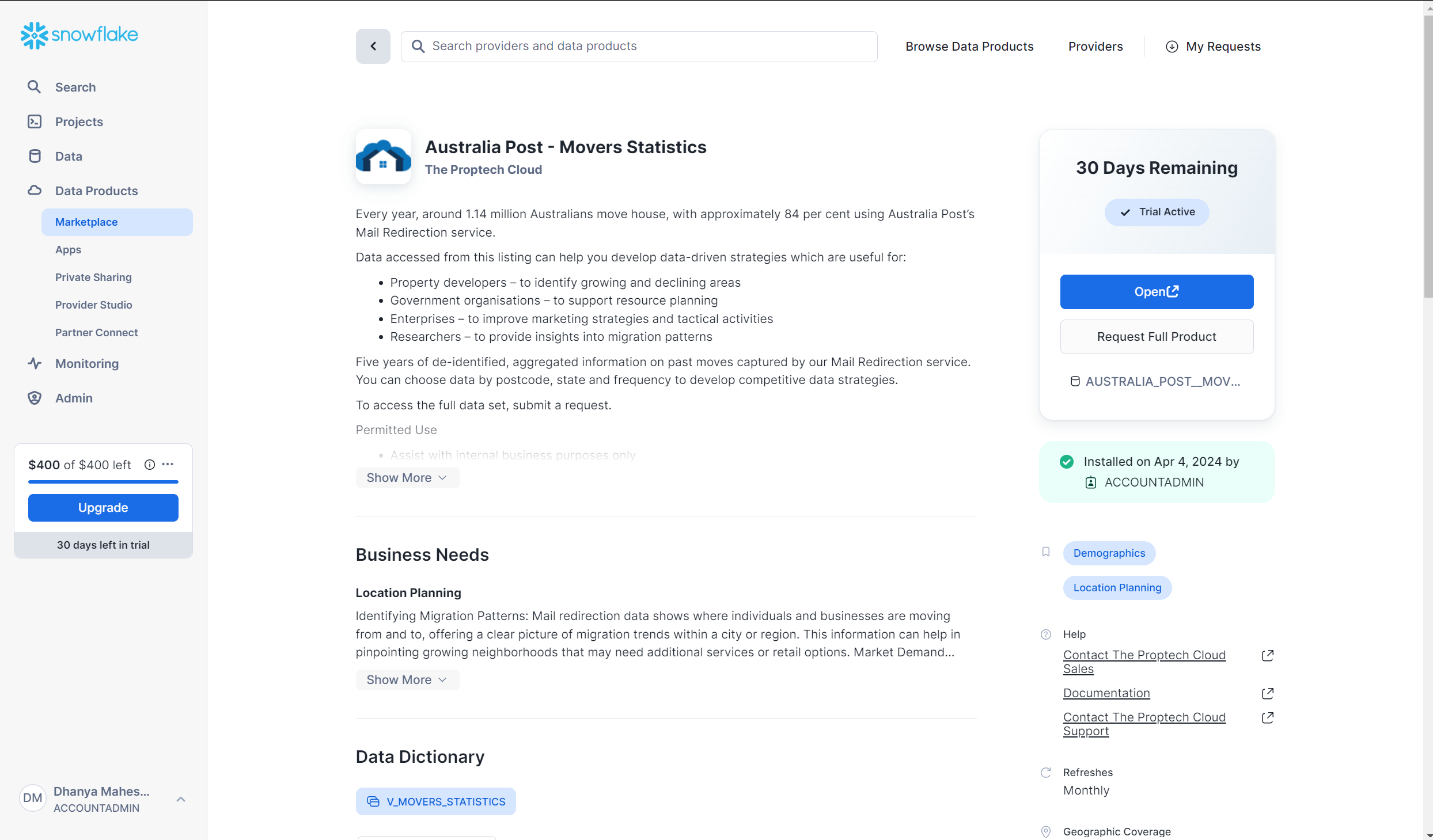
  4. Once your Snowflake account is set up and running , the Australia post Mover Statistics dataset listing is located within Data Products and then Marketplace as shown by the link below:
Snowflake Marketplace screen

5. Click on the Open button to explore the sample data within the Snowflake Environment. This will redirect to a Snowflake worksheet which will show some sample queries.

6. The full product can also be requested from the Marketplace page with the button ‘Request Full Product’ if access to the entire dataset is needed.

Step 2: Setting Up the Example Data

The forecasting model created is a multi-time-series model. The following types of variables were needed to create this:

  • The series variable to create multiple time series forecasting
  • A timestamp column
  • A target column which includes a quantity of interest at each timestamp

The cleaning and transformation of the dataset to prep the data for forecasted was completed by running SQL queries using Snowpark. A sample of this data is shown below:

Snowflake Marketplace - tables
This data is then saved as a view named migration_people_moving_to to use in the forecasting model.

Step 3: Creating the Forecasting Model

Each row in the migration_people_moving_to view corresponds to the three types of columns needed to create a multi-series forecasting model; the postcode (series column), month (timestamp column) and the number of people who moved into the postcode that month (the target column)

The code to create a forecasting model is as follows:

CREATE OR REPLACE SNOWFLAKE.ML.FORECAST forecasting_model_people_to (

INPUT_DATA => SYSTEM$REFERENCE('VIEW', 'migration_people_moving_to'),

SERIES_COLNAME => 'to_postcode',

TIMESTAMP_COLNAME => 'timestamp_month',

TARGET_COLNAME => 'number_of_people_to_postcode'

)

This will create the forecasting model forecasting_model_people_to

Step 4: Calling and Interpreting the Forecasting Model

The model can then be used to forecast for any number of periods in the future. The model will perform better for forecasting periods that are closer training dataset, and are less reliable when it is used to forecast for periods further into the future.

The code used to forecast the number of people moving into a postcode every month for 12 months and save it to a table is shown below.

BEGIN

CALL forecasting_model_people_to!FORECAST(FORECASTING_PERIODS => 12);

LET x := SQLID;

CREATE OR REPLACE TABLE forecast_12periods_move_to AS

SELECT * FROM TABLE(RESULT_SCAN(:x));

END;

An example of the forecasting model output results are shown below.

Snowflake Marketplace - forecasting model output results

The way to interpret the above output would be to say that the number of people forecasted to move into Postcode 5096 (which covers Para Hills, Para Hills West, Gulfview Heights, Adelaide) in April 2024 is approximately 26. The lower bound and upper bound of 12.6 and 38.7 represent the prediction interval. For the April 2024 forecast into Para Hills, the model is 95% confident that the number of people who will move into postcode 5096 in April 2024 is between 12.6 and 38.7. A smaller prediction interval indicates that there is less error in the model and the estimated forecast is more likely to be accurate and vice versa.

The default prediction interval when calling a model in Snowflake is 95%. However, this can be configured when calling the model by adding a prediction interval. The code below shows how to call a model with an 80% prediction interval:

CALL forecasting_model_people_to!FORECAST(FORECASTING_PERIODS => 12, CONFIG_OBJECT => {'prediction_interval': 0.8})

Step 5: Visualising the forecasts using Snowpark and Streamlit

The 12 months results of the forecasting model were then aggregated to produce the total of number people forecasted to move into each postcode across Australia.

The data was then also joined with the Australian Postcode boundaries from the Geography Boundaries & Insights – Australia to allow for geospatial visualisations.

The visualisations were hosted using Streamlit within the Snowflake User Interface.

Streamlit is an open source python library which allows for the creation and sharing of data web applications. Using Streamlit within the Snowflake console allows for the flexibility to securely clean, transform and visualise the data in one place, without the need for any external environments.

Data Visualisation – Greater Melbourne Region

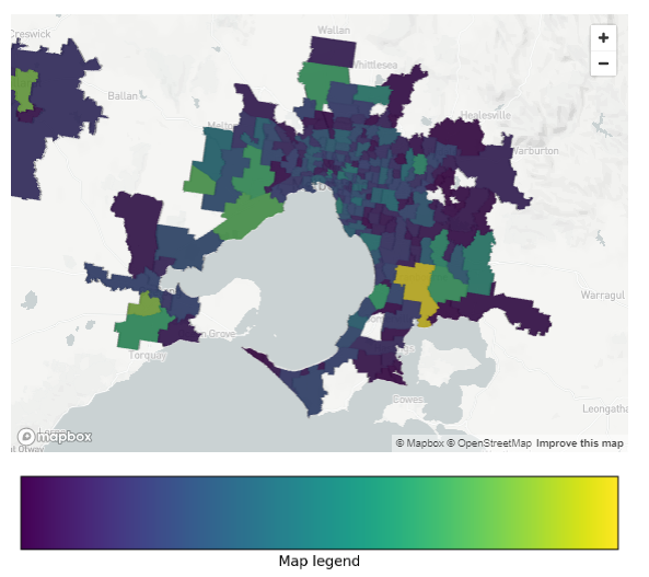
The visualisation shows the postcodes that people are moving to in the Greater Melbourne region.

The green and yellow regions show the places where high numbers of people are forecasted to move into in the next year, while the purple and blue regions show the regions that are forecasted to have a lower amount of relocation in the next year.

Interestingly, the visualisation shows that places in the outer East including Cranbourne, Clyde North and the outer west including Point Cook and Werribee South. The inner city postcodes which include suburbs such as Fitzroy, Brunswick and North Melbourne are forecasted to have much less migration in the next year.

Streamlit - Data Visualisation of migrations
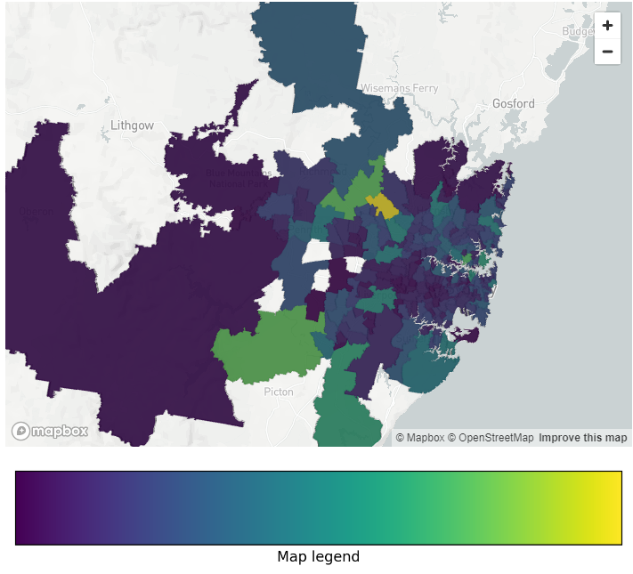
Streamlit - Data Visualisation of migrations SYD

Data Visualisation – Greater Sydney Region

A similar visualisation was done in the Greater Sydney area, where a similar trend was observed.

High levels of migration are forecasted for outer-city areas including Kellyville and North Kellyville and outer-city south west south west areas including Camden and Oran Park.

Like Melbourne, there seems to be less migration forecasted for inner city suburbs including Chippendale, Ultimo and Redfern.

Steps to Create the Visualisations

The following steps were performed to create the geospatial visualisations.

Firstly, the base steps to create a Streamlit App were completed. This includes creating an app and selecting a warehouse to run the queries. This will then create a Snowpark worksheet which allows the creation of a Streamlit app using Python. The Streamlit environment also needs to be set up to allow for the ingestion of packages which requires the CREATE STREAMLIT permission.

The third-party packages were then ingested using the Packages tab at the top of the worksheet. Only packages which are supported by Snowflake are able to be ingested to ensure that the Snowflake platform remains secure. Both Matplotlib and Pydeck were ingested to create these visualisations.

The required packages were then imported to create the Streamlit visualisation

# Import python packages

import streamlit as st

from snowflake.snowpark.context import get_active_session

import json

import pydeck as pdk

import matplotlib.pyplot as plt

import matplotlib as mpl

The Snowpark package was used to connect the worksheet to the table containing the 12 month forecasting data in Snowflake. The postcode geospatial boundaries were also obtained, joined to the forecasting data and converted into a geojson format. This was achieved using the code below:

session = get_active_session()


session.sql ("""SELECT
POA_CODE_2021 as POSTCODE_NAME,
NUMBER_OF_PEOPLE,
ST_ASGEOJSON(geometry) AS geojson
FROM
forecast_12periods_move_to --forecasting model table created in Step 3
INNER JOIN ABS_POA_2021_AUST_GDA2020
ON POA_CODE_2021 = TO_POSTCODE
""").collect()

Each row in the query represents the postcode, the number of people forecasted to move into the postcode in the next year and a geojson representing to geometry of the postcode boundary. Further transformations were done on the result so that each row in the query result was transformed into a dictionary. A key aspect of this transformation was assigning RGB colour code to each postcode depending on the number of people forecasted to migrate to that postcode. A sample of the geojson format is shown below:

map_geojson = {
"type": "FeatureCollection",
"features":[
{"type": "Feature",
"properties":
{"postcode": 2000,
'colour':(68, 1, 84)
},
"geometry":{'geometry in geosjon format'}
},
{"type": "Feature",
"properties":
{"postcode": 2000,
'colour':(38, 130, 142)
},
"geometry":{'geometry in geosjon format'}
},
]
}

The base chloropeth map was then set up by assigning the centre and zoom point for the map to render.

pydeck_chloropeth = pdk.Deck(
map_style=None,
initial_view_state=pdk.ViewState(
latitude={insert centre latitude},
longitude={insert centre longitude},
zoom={insert zoom level},
),

The geojson created in the step above was then added to the base map to create the chloropeth layer using the code below.

layers=[
pdk.Layer(
"GeoJsonLayer",
map_geojson, #name of the goejson created earlier
opacity=0.8,
stroked=False,
filled=True,
extruded=True,
wireframe=True,
get_fill_color='properties.colour',
get_line_color=[255, 255, 255],
)

],
)

The legend on the map was created using the colorbar function in the matplotlib library.

fig, ax = plt.subplots(figsize=(6, 1), layout='constrained')

cmap = mpl.cm.viridis
norm = mpl.colors.Normalize(vmin=0, vmax=1)

fig.colorbar(mpl.cm.ScalarMappable(norm=norm, cmap=cmap),
cax=ax, orientation='horizontal', label='Map legend', ticks=[])

Finally, the following lines of code were used to render both the chloropeth map and the legend on the Streamlit app.

st.pydeck_chart(pydeck_chloropeth)
st.pyplot(fig)

Summary

In this blog, the Australia Post Movers Statistics Marketplace listing was used along with Snowflake’s Cortex ML Forecasting function to forecast the postcodes within Australia that have high levels of population movement.

The Streamlit data visualisations revealed that the postcodes that the highest amount of people were forecasted to move into were predominantly located in the outer-city area. Read our following blog to understand where people are moving to.

The rundown above highlights how the Snowflake Data Platform makes it straightforward for businesses to access quality data and market-leading compute, AI and visualisations all on one neat platform.


Australia Post Movers Statistics Data

This dataset contains five years of de-identified, aggregated information on past moves captured by Australia Post’s Mail Redirection service.

Access Australia Post mail redirect statistics now to help you develop competitive data-driven strategies.

The intellectual property rights for all content in this blog are exclusively held by Data Army and The Proptech Cloud. All rights are reserved, and no content may be republished or reproduced without express written permission from us. All content provided is for informational purposes only. While we strive to ensure that the information provided here is both factual and accurate, we make no representations or warranties of any kind about the completeness, accuracy, reliability, suitability, or availability with respect to the blog or the information, products, services, or related graphics contained on the blog for any purpose.

Subscribe to our newsletter

Subscribe to receive the latest blogs and data listings direct to your inbox.

Read more blogs from The Proptech Cloud

Australia’s Migration Trends: Where Are People Moving To?

This detailed visual analysis for Australia’s major capital cities breaks down how net migration trends are evolving across different regions.

How to Predict Migration Patterns using Auspost Movers Statistics Data and Snowflake’s Cortex ML functions

How to predict the Australia postcodes people are most likely to relocate to using the Australian Post Movers Statistics dataset and Snowflake Time Series Forecasting function.

Could a Revamp of Australian Property Planning Rules Solve Some of Australia’s Housing Issues?

Rising property prices and high costs of living means the Australian dream of home ownership is slipping further away for many. Could the answer lie in a revamp of property planning rules?

Top Real Estate Technology Global Events

Staying abreast of the latest trends, technologies, and innovations is crucial for professionals seeking to leverage the full potential of real estate technology and proptech.

What Are Mesh Blocks & How Are They Used in Real Estate

What are Mesh Blocks? As defined by Australian Bureau of Statistics (ABS), mesh blocks are the smallest geographical area of the Australian Statistical Geography Standard (ASGS) and ABS’s classification of Australia into a hierarchy of statistical areas. Mesh Blocks...

Building a Rental Property Automated Valuation Model (AVM)

Building a Rental Property Automated Valuation Model (AVM)

A Rental Automated Valuation Model (AVM) serves as an indispensable tool for a myriad of stakeholders within the property ecosystem.

Besides businesses managing extensive rental portfolios, real estate portals, valuers, banks, and proptech companies, it can also benefit insurance firms, property developers, and governmental housing authorities.

What is a Rental Property Automated Valuation Model?

A rental property automated valuation model (AVM) is a tool which estimates the rent and yield of a property.

What are the Benefits of Owning a Rental Property AVM?

Rental Property AVM

Owning a rental AVM provides a competitive edge through real-time valuation insights, which facilitates informed decision-making regarding rental pricing, portfolio management, and investment strategies.

The benefits of owning a rental AVM extend to enhanced accuracy in rental appraisals, time and cost efficiency, and the ability to customise the model to align with specific business objectives and market dynamics. It paves the way for data-driven strategies, fostering a deeper understanding of market trends and rental property performance.

Therefore, a cautious approach is paramount. Businesses should meticulously evaluate the financial, operational, and regulatory implications before embarking on the development of a rental AVM. A thorough understanding of the costs involved in building, owning, and maintaining such a model is crucial to ascertain the long-term viability and to mitigate the risks associated with this substantial investment.

Embarking on the construction of a Rental Property Automated Valuation Model (AVM) necessitates a well-structured foundation that ensures precision, reliability, and effectiveness in valuing rental properties.

Core Requirements for Building a Rental Property AVM

  1. Address Database:
    A comprehensive address database is indispensable as it serves as the primary reference point for rental properties.
    Each address should have a unique identifier to ensure no duplication or confusion arises in the data.
  2. Geocoding Addresses:
    Geo-coding the addresses is crucial for pinpointing the exact geographical location of each rental property.
    This geo-spatial information is pivotal for applying distance measures which are integral in comparative analysis and valuation.
  3. Back-series Data:
    Accumulating back-series data, ideally spanning at least three years, is fundamental for a nuanced understanding of rental market dynamics over time. Records should include address, property type, rental price, rental date, beds, baths and parking at a minimum.
    This historical data permits the creation of an index to track rental values through time, which is invaluable in comparative market analysis.
    Additionally, back-series data serve as inputs for regression models and machine learning algorithms, providing coefficients essential for adjusting rental prices in a virtual rental comparative market analysis.
  4. IT Resource:
    A proficient IT resource is necessary for building, deploying, and maintaining the database and the rental AVM model.
    They would be responsible for ensuring system efficiency, security, and scalability, ensuring the model adapts to the evolving market dynamics.
  5. Database Resource:
    A dedicated database resource is required to manage the vast amount of data involved in this project.
    They ensure data integrity, accuracy, and availability, which are crucial for the reliability of the AVM.
  6. Organisational Commitment:
    It’s imperative that the organisation has a firm commitment to provide the necessary resources for the successful completion of this project. In the absence of requisite IT and database resources, it might be prudent to reconsider the viability of this project.
Rental Property AVM

Checklist

  • Acquire a comprehensive address database.
  • Implement geocoding for all addresses.
  • Collect a minimum of three years’ worth of back-series data.
  • Secure a skilled IT resource for system development and maintenance.
  • Have a dedicated database resource for data management.
  • Evaluate organisational resource availability and commitment to the project.

This section lays the groundwork for what is needed to commence the journey towards creating a robust Rental Property Automated Valuation Model. Each requirement is pivotal and necessitates careful consideration and planning.

Typical Build Requirements for Rental Automated Valuation Model (AVM)

Creating a reliable and efficient Rental Automated Valuation Model (AVM) necessitates a meticulous approach towards the build requirements. Here’s a high-level outline of the components and processes involved:

  1. Database:
    Establishing a robust database to store and manage the diverse set of data involved in the valuation process.
  2. Index:
    Creating an index to track and compare rental values over time.
  3. Weekly Rental Data Source:
    Securing a reliable source of weekly rental data to keep the model updated with current market conditions.
  4. ETL Process:
    Designing an Extract, Transform, Load (ETL) process to handle rental data, including filtering, standardisation, duplicate removal, and data hierarchy management.
  5. Address and Geospatial Service:
    Ensuring an ongoing service for address verification and geospatial data.
  6. Reports:
    Generating reports encompassing medians, data management records, and dashboards for insightful analysis. This should also include error reports.
  7. Lookups:
    Developing lookup functions to standardise and categorise data fields, aiding in data accuracy and consistency.
  8. Outlier Management:
    Implementing systems to identify and manage outliers and influential observations, preventing erroneous data entry.
  9. Model Framework:
    Creating a framework to index the last rental price and to match comparable rentals automatically, akin to a rental Comparative Market Analysis (CMA).
  10. Machine Learning Integration:
    Incorporating machine learning functions to test and adjust model iterations per suburb or locale, ensuring precise valuation.
  11. Extended Features:
    Adding features like street details and information about strata buildings to enhance the model’s accuracy and comprehensiveness.
  12. Regular Training:
    Implementing a regular training schedule to keep the model updated and improve its predictive accuracy over time.

This outline is designed to provide a clear roadmap towards building a robust Rental AVM. While not exhaustive, it encompasses the critical aspects that require consideration to ensure the successful deployment and operation of the model.

Each of these components will be elaborated upon in the subsequent sections, providing a deep dive into the intricacies involved in each stage of the development process.

Part 1: Database Construction for Rental AVM

The cornerstone of developing a robust Rental Automated Valuation Model (AVM) is the establishment of a comprehensive and well-structured database.

This database will serve as the repository of all pertinent information required to perform nuanced and accurate rental valuations. Here are some critical considerations and steps involved in setting up the database:

  1. IT Resource with Property Database Skills: Having an IT resource with expertise in property databases is indispensable for this endeavour. The intricate nature of property data and the rental market dynamics necessitate a deep understanding and skilled handling of the data.
  2. Utilisation of Geoscape Database: In Australia, leveraging the government-maintained Geoscape database could serve as an ideal foundation due to its comprehensive property data schema. This database encompasses critical geospatial and address information which is paramount for accurate rental valuations.
  3. Incorporation of Rental Data Tables: Rental data tables should be meticulously designed and integrated within the Geoscape schema or an alternative robust schema. These tables will hold the rental data, both current and historical, for each property.
  4. Time-Series Data Storage: A common pitfall for novices is the improper handling of time-series data. It’s crucial to design the database such that the same property record can be stored through time, capturing all rental transactions and changes in property attributes.
  5. Derivative Metrics and Indexation: Storing all time-series and historical data facilitates the creation of derivative metrics and indices. These metrics, like indexation, provide insightful trends and comparative measures for rental valuations.
  6. Comprehensive Attribute Storage: The database should accommodate the storage of a plethora of attributes for each rental. This includes not only the rental price history but also details about the address, street, building, and locale data.
  7. Data Integrity and Consistency: Ensuring data integrity and consistency is paramount. Implementing stringent data validation and verification processes will aid in maintaining a high level of data accuracy.
    A well-architected database is the bedrock upon which the other components of the Rental AVM are built. It requires a meticulous design, skilled resources, and an ongoing commitment to data management to ensure the reliability and accuracy of the rental valuations generated by the AVM.

Part 2: Index Construction for Tracking and Comparing Rental Values

Creating an index is a fundamental aspect of a Rental Automated Valuation Model (AVM) as it provides a mechanism to track and compare rental values over time, thereby offering a quick and effective way to update rental prices to reflect current market conditions.

Here are the key considerations and methods involved in index construction:

  1. Instantaneous Price Updating: The index enables immediate price updating based on the last advertised rent or the last rental Comparative Market Appraisal (CMA), aligning the prices with the current market trend.
  2. Monthly Database Indexing: Each month, the entire database and portfolio are indexed to ensure the rental values remain relevant and reflective of the prevailing market dynamics. This method remains effective typically for up to 3 or 4 years.
  3. Automated CMA Adjustment: The index adjusts the comparative rentals used in the automated CMA, facilitating the matching of nearby rentals for up to 12 months while ensuring the price estimate remains in sync with market movement.
  4. Median-Based Indexing: One simplistic approach to index construction is utilizing the median rental value for a given area. In Australia, medians are often measured at a Statistical Area 3 (SA3) basis, which can be imported and utilized directly, or recalculated as needed. This approach can extend to smaller areas like SA2 or suburb level, provided there’s a significant rental sample each month to mitigate excessive volatility.
  5. Property Type Segmentation: It’s imperative to measure the median after categorising rentals by logical property types such as houses (including terraces) and units (including apartments, townhomes, flats, and villas). Further subdivision into sub-market groups may be feasible depending on the location and data availability.
  6. Repeat-Rental Indexing: Another nuanced approach involves tracking the change over time of repeat rentals. In a design akin to a repeat-rental-index, rentals with two prices spanning 1 to 5 years are entered into the model. This method, albeit more complex, could provide a deeper insight into rental value trends and may be worth exploring depending on the project scope and budget.
  7. Custom Index Calculation: For those with adequate resources, developing a custom index at a more granular level could provide more precise and tailored insights, aiding in a more accurate rental AVM. The construction of a robust index is a nuanced process that requires a strategic approach. Whether opting for a median-based index or exploring the repeat-rental indexing method, the goal is to ensure the index accurately captures the rental market dynamics, aiding in the effective operation of the Rental AVM.
Rental Property AVM

Part 3: Procurement of Weekly Rental Data Source

Ensuring a consistent and reliable source of weekly rental data is paramount for the effective operation and accuracy of a Rental Automated Valuation Model (AVM).

A diligent update on a weekly basis keeps the model attuned to the prevailing market conditions, thereby enhancing the precision in rental valuations.

Here are some key considerations:

  1. Data Relevance: Advertised rentals have long served as a credible source for rental price models and are widely recognised in the industry. Alternatively, some advocate for using final contracted rental prices, although procuring such data on a national scale may pose challenges. Either of these data sources can be utilised based on availability and project requirements.
  2. Data Attributes: The rental data procured should comprehensively capture crucial attributes including:
    Full address (preferably pre-geocoded).
    Property type (requiring standardisation via lookups in most cases).
    Number of bedrooms, bathrooms, and parking spaces.
    Rental date and rental price.
  3. Geocoding and GNAF PID Matching (for Australia): In the Australian context, matching the address to a Geocoded National Address File (GNAF) PID is beneficial for ensuring precise location identification.
  4. Unique Identifier Establishment: While the address serves as a primary identifier, it’s vital to distinctly identify the street and strata (apartment) building, which can act as unique matching identifiers aiding in accurate data matching and analysis.
  5. Standardisation: Standardising data, especially the property type, through lookups ensures consistency across the dataset, which is critical for accurate comparative analysis and valuation.
    This procurement and structuring of weekly rental data form the crux of maintaining a dynamic and responsive Rental AVM, allowing for real-time insights and a thorough understanding of the rental market trends.

Part 4: Designing a Robust ETL Process for Rental Data Management

The Extract, Transform, Load (ETL) process is a critical pillar in the data management framework of a Rental Automated Valuation Model (AVM). It ensures that rental data is accurately harvested, refined, and loaded into the database for optimal utilisation.

Below are the key components and considerations in designing an effective ETL process:

  1. Duplicate Handling: An efficient mechanism to identify and handle duplicates is crucial to maintain data integrity. When the same record is collected from different sources, a hierarchy or trust rating system should be in place to select the more reliable source.
  2. Data Standardisation: Rental data often requires standardisation, especially when it comes to free-text fields. Utilising tools like ChatGPT can significantly aid in converting free-text data into a structured and standardised format.
  3. Data Filtering: Implementing filters to weed out irrelevant or erroneous data is essential to ensure the quality and reliability of the information being loaded into the database.
  4. Local Expertise: In Australia, leveraging local expertise in the ETL domain can expedite the deployment of a fit-for-purpose ETL solution for real estate data, bypassing the steep learning curve associated with standard ETL tools.
  5. Customised ETL Solution: Although off-the-shelf ETL tools are an option, a customised solution tailored to handle real estate data peculiarities can be more beneficial in the long run. This can be achieved by collaborating with experts who have a deep understanding of the Australian real estate data landscape.
  6. Continuous Learning and Improvement:  The ETL process will likely require fine-tuning over time. Learning from the data handling experiences and continuously improving the ETL process is pivotal for achieving and maintaining a high level of data accuracy and efficiency.

The design and implementation of a robust ETL process is a meticulous task that demands a blend of the right technology, expertise, and a thorough understanding of the real estate data ecosystem. This ensures that the rental AVM operates on a foundation of accurate, reliable, and well-structured data.

Part 5: Address and Geospatial Service Integration

A dedicated service for address verification and geospatial data management is indispensable in refining the accuracy and reliability of a Rental Automated Valuation Model (AVM).

Below are pivotal considerations and tools:

  1. Address Verification: Utilising Australia’s Geocoded National Address File (GNAF) is an exemplary method for precise address verification. However, third-party services also offer valuable solutions for rectifying poor quality addresses collected via free text inputs.
  2. Geospatial Data Layer: Incorporating a geospatial layer enhances the model’s efficiency in matching comparable properties by providing spatial insights. It aids in better understanding the proximity and locational advantages of properties, which are crucial factors in rental valuations.
  3. Data Repair and Standardisation: Leveraging services that can repair and standardise address data is vital to ensure consistency and accuracy in the database. This is particularly important when the initial data collection may have inconsistencies due to free text entries.
  4. Continuous Service: Engaging a continuous service for address and geospatial data management ensures the model remains updated with accurate locational data, aiding in the precise valuation and comparison of rental properties.

The integration of robust address verification and geospatial data services fortifies the model’s foundation, ensuring precise and meaningful insights in rental valuation and comparative analysis.

Part 6: Report Generation for Insightful Analysis and Performance Monitoring

Generating comprehensive reports is a vital component in the management and continuous improvement of a Rental Automated Valuation Model (AVM).

These reports provide a clear picture of the model’s performance, data management efficiency, and areas requiring attention.

Key considerations include:

  1. Error Reporting: Essential error reports like Forecast Standard Deviation (FSD) and Percent Predicted Error (PPE10) provide invaluable insights into the accuracy of rental valuations. For instance, calculating the percentage and dollar value error as a new rental record enters the database facilitates immediate performance assessment. Records with AVM estimates within 10% of the actual rental price can be flagged, enabling the calculation of properties estimated within a 10% accuracy range, which can be reported by property type, suburb, or broader geographical areas.
  2. Median, Volume, and Hit-Rate Reporting: Reports displaying median rental values, the volume of rental records entering the database, and the hit-rate (the proportion of records for which an AVM can be generated) are crucial for evaluating data management efficiency and model coverage.
  3. Dashboard Creation: Designing dashboards that encapsulate key metrics provides a succinct overview of the model’s performance, aiding in prompt decision-making and continuous improvement.
  4. Monthly Tracking: Monthly tracking of error rates, hit-rates, and other key metrics enables trend analysis, which is instrumental in identifying areas of improvement and assessing the impact of any modifications made to the model.
  5. Customised Reporting: Tailoring reports to meet specific organisational needs ensures that the insights generated are aligned with the objectives and requirements of managing the rental AVM effectively.

Through diligent report generation and analysis, stakeholders can maintain a firm grasp on the model’s performance, the quality of data management, and the accuracy of rental valuations, which are integral for the successful operation and continuous refinement of the Rental AVM.

Rental Property AVM

Part 7: Lookups: Enhancing Data Accuracy and Consistency

Implementing lookup functions is a pivotal step in managing the database effectively, ensuring data standardisation, and categorising data fields to bolster accuracy and consistency in a Rental Automated Valuation Model (AVM).

Here are some critical aspects and benefits of developing lookup functions:

  1. Standardisation of Property Types: Different regions or states may employ varied standards for defining property types. Lookup tables can harmonise these discrepancies by mapping varied definitions back to a standard classification, ensuring uniformity across the dataset.
  2. Correction of Free Text Errors: Free text entries are prone to inconsistencies and errors. Lookup functions can be employed to identify common errors and rectify them, thereby enhancing the quality of data.
  3. Utilisation of ChatGPT: Leveraging ChatGPT can expedite the setup and maintenance of lookups significantly. With its capability to process and standardise free text, ChatGPT serves as a valuable tool in automating the correction of common errors and inconsistencies, thereby reducing manual effort and enhancing accuracy.
  4. Dynamic Error Correction: Over time, new errors or discrepancies may emerge. A dynamic lookup function, aided by ChatGPT, can adapt to new patterns, facilitating ongoing data quality maintenance.
  5. Enhanced Database Management: Lookup functions contribute to a structured and well-managed database, which is foundational for generating accurate rental valuations and insightful analysis.
  6. Support for Automated Processing: Lookups support automated data processing by ensuring data fields are standardised and categorised correctly, which is crucial for the efficient operation of the AVM.
  7. Reduced Data Cleaning Overheads: By automating the process of error correction and standardisation, lookups reduce the time and resources required for data cleaning, enabling a more streamlined and efficient database management process.
  8. Improved Model Performance: Standardised and accurate data significantly contribute to the overall performance and reliability of the rental AVM, ensuring that the valuations generated are reflective of the actual market conditions.

The development and continuous refinement of lookup functions are instrumental in fostering a high level of data integrity and operational efficiency in managing the rental AVM.

Part 8: Outlier Management: Safeguarding Against Erroneous Data Entry

Rental Property AVM

Effective outlier management is crucial to maintain the integrity and accuracy of a Rental Automated Valuation Model (AVM).

Outliers and influential observations, if not handled appropriately, can lead to skewed valuations and misrepresentations of the rental market.

Here’s how to approach outlier management:

  1. Identification of Outliers: Outliers can be spotted based on extreme rental price values. Utilising the 1.5*Interquartile Range (IQR) rule is a standard measure, but it’s essential to apply this rule carefully to prevent inadvertent removal of valid records.
  2. Sampling Strategy: Employing a well-thought-out sampling strategy, such as examining a suburb sample over 12 months by property type, is crucial. A carefully curated sample minimises the risk of erroneously identifying valid records as outliers.
  3. Multivariate Analysis: Incorporating multivariate analysis helps in identifying records that significantly impact the model performance upon their entry into the rental AVM. This approach is vital in spotting observations that may skew the model outcome.
  4. Influential Observation Metrics: Measures such as Cook’s Distance are standard for identifying influential observations. Integrating such metrics into the model aids in recognising and managing observations that could disproportionately affect model performance.
  5. Automated Outlier Detection: Developing automated systems for outlier detection and management can enhance efficiency and accuracy in maintaining data quality. It also ensures a timely response to erroneous data entries.
  6. Continuous Monitoring and Adjustment: Continuous monitoring and adjustment of the outlier management system is crucial to keep pace with evolving data trends and to ensure the ongoing effectiveness of the outlier detection mechanisms.
  7. Documentation and Review: Documenting outlier occurrences and reviewing the outlier management processes regularly provide insights for improvement and ensure a clear understanding of the model’s performance dynamics.
  8. Integration with Reporting: Integrating outlier management insights into the reporting framework provides a comprehensive view of data quality and model performance, enabling informed decision-making and continuous improvement.

By adopting a meticulous approach to outlier management, the robustness and reliability of the Rental AVM are significantly enhanced, ensuring that the valuations generated are a true reflection of the rental market conditions.

Part 9: Developing a Robust Model Framework for Rental AVM

The creation of a model framework for a Rental Automated Valuation Model (AVM) is a nuanced undertaking that goes beyond just feeding massive datasets into machine learning models.

It entails crafting a systematic approach that mirrors the methodical selection of comparable rentals, akin to a rental Comparative Market Analysis (CMA), while also ensuring accurate indexation of the last rental price.

Here’s an outline of the core components and considerations in developing such a framework:

  1. Matching Algorithm Design: The foundation of the model is the creation of a matching algorithm that accurately pairs comparable rentals to the subject property. This algorithm takes into account variables such as time, distance, bedroom count, bathroom count, and parking availability. A perfect match scores 100%, with a desirable match rate being 70% or better. The weights assigned to each variable in the matching algorithm can be fine-tuned at a suburb, postcode, or even broader geographical level, and further boosted for comparables within the same street or building.
  2. Utilisation of Advanced Tools: The advent of advanced tools like ChatGPT significantly enhances the model, especially when enriched with geospatial data, images, text, or maps. Even preliminary tests with ChatGPT have shown promising results in refining the matching algorithm, indicating a potential for substantial model improvement.
  3. Grid Adjustment Coefficients: This aspect of the model accounts for adjustments needed over time, or for differences in bedroom, bathroom counts, and parking availability. Additional variables like floor levels and aspect could be integrated in select scenarios. These coefficients can be stored as either dollar values or percentages, with percentages often proving more robust.
  4. Continuous Training and Refinement: The matching scores and grid adjustment coefficients should be subjected to continuous training, testing, and refinement, exploring thousands of permutations to enhance accuracy. This iterative process can be expedited using ChatGPT or standard statistical code, aiding in the monthly or periodic retraining of the model.
  5. Professional Deployment and Maintenance: Storing the matching coefficients in database tables and ensuring professional deployment and maintenance of the model is crucial for sustaining its performance and reliability.
  6. Avoidance of Overfitting: Steering clear of overfitting by embracing model designs evolved over years, which emulate appraiser or real estate agent methodologies in selecting comparables, is imperative to prevent catastrophic model failures.

This structured approach to developing a model framework not only aligns with traditional appraisal methodologies but also harnesses modern tools to significantly enhance the accuracy and reliability of the Rental AVM.

Part 10: Integrating Machine Learning for Precise Valuation in Rental AVM

The infusion of machine learning (ML) into the Rental Automated Valuation Model (AVM) framework presents an avenue for enhancing valuation precision across different suburbs or locales.

While ML facilitates rapid model deployment, a siloed ML approach often falls short due to overfitting and lack of inclusivity in a broader model framework.

Moreover, the opacity of ML models, where the specific comparables used for a rental property estimate remain unidentified, poses a challenge.

The common reflex to attribute poor model results to inadequate data further underscores the limitations of a standalone ML approach.

  1. Enhancing Traditional AVMs: The integration of ML into time-tested, industrial-grade AVMs, honed over two to three decades, offers a pragmatic solution. This fusion capitalises on the strengths of both ML and traditional AVM methodologies, mitigating the shortcomings of a solitary ML approach.
  2. ChatGPT Integration: Incorporating ChatGPT, an advanced tool, into the AVM framework can significantly augment the matching scores and functionality. It opens new vistas for processing and utilising data beyond existing quantitative measures, thereby pushing the boundaries of what can be achieved in rental valuation precision.
  3. Transparent ML Approaches: Exploring ML approaches that offer a level of transparency, and integrating them with existing AVM frameworks, can provide a more comprehensive, understandable, and reliable rental valuation model.
  4. Continuous Evaluation and Adjustment: Regularly evaluating the ML-integrated AVM, and making necessary adjustments based on the insights garnered, is crucial to maintain the model’s accuracy and relevance in a dynamic rental market.
  5. Collaborative Development: Encouraging a collaborative milieu between ML practitioners, real estate experts, and AVM developers can foster the creation of more robust, transparent, and effective rental valuation models.

In summary, a judicious integration of ML, especially with tools like ChatGPT, into established AVM frameworks can herald a significant leap in achieving precise and reliable rental valuations, while overcoming the inherent limitations of a standalone ML model.

Part 11: Extended Features: Enriching Model Accuracy and Comprehensiveness

Introducing extended features such as street details and information about strata buildings enriches the Rental Automated Valuation Model (AVM), amplifying its accuracy and comprehensiveness. Here’s an exploration of how these extended features and new data sets can be integrated to enhance the model:

  1. Population-Level Data: The value of new data is often directly proportional to its coverage across properties. Data at or near population level, applicable across all properties, is deemed more valuable as it provides a comprehensive enhancement to the model.
  2. Strata Buildings and Street Details: Detailed information about strata buildings and street-level data provide nuanced insights that refine rental valuations. They account for variables like the desirability of a location, the quality of local infrastructure, and the proximity to amenities, which are critical for precise rental appraisals.
  3. ChatGPT and AI Integration: The integration of ChatGPT and AI technologies unlocks the potential to process and utilise diverse data sets like mapping and geospatial data, free text, and images. This integration paves the way for extracting valuable insights from unconventional data sources.
  4. Geospatial Data: Geospatial data can provide crucial contextual information regarding a property’s location, proximity to essential amenities, and the overall desirability of the area, significantly impacting rental valuations.
  5. Free Text and Image Analysis: Utilising ChatGPT for processing free text and image data can help in extracting valuable information that can be integrated into the model. For instance, textual descriptions or images from rental listings can provide insights into a property’s condition, features, and appeal.
  6. Exploration of New Data Sets: Continuous exploration of new data sets, especially those available at a broader scale, is essential. Evaluating the impact of these data sets on model performance ensures that the model remains robust and reflective of current market conditions.
  7. Iterative Enhancement: An iterative approach to integrating and evaluating extended features ensures that the model evolves in line with advancements in data availability and technology.

In essence, the incorporation of extended features, leveraged through advancements in AI and tools like ChatGPT, presents an avenue for elevating the accuracy, reliability, and comprehensiveness of the Rental AVM, thereby ensuring that it remains a robust tool for rental valuation in a dynamic real estate market.

Part 12: Regular Training: Ensuring Optimal Model Performance Over Time

A systematic schedule for regular training is pivotal for maintaining and enhancing the predictive accuracy of the Rental Automated Valuation Model (AVM).

Models are susceptible to degradation over time due to evolving market conditions, hence the imperative for periodic re-tuning and re-training using updated data sets. Here are the key considerations and steps for implementing a regular training schedule:

  1. Data Sample Selection: Careful selection of the data sample for training is crucial. A bias towards more recent data is advisable, yet attention must be paid to ensuring sufficient sample sizes to avoid statistical anomalies.
  2. Handling Outliers and Influential Observations: Vigilant management of outliers and influential observations is essential to prevent deleterious impacts on the model. These can skew the training process and lead to inaccurate predictions.
  3. Geographical Area Selection: In instances where suburb samples are too sparse, expanding the geographical area for data sampling is a prudent step to ensure a robust training process.
  4. Continuous Performance Monitoring: Regular performance monitoring, facilitated through comprehensive reporting, enables tracking of model performance over time. This is crucial for diagnosing issues and understanding the impact of market shifts on the model.
  5. Adaptive Training Schedules: The training schedule should be adaptive to the model’s performance and the availability of new data. This flexibility ensures the model remains attuned to the current market conditions.
  6. Utilisation of Updated Technologies: Employing updated technologies and methodologies for the training process ensures the model benefits from the latest advancements in data processing and machine learning.
  7. Performance Evaluation: Post-training evaluation is vital to ascertain the effectiveness of the training process, and to identify areas for further improvement.
  8. Feedback Loop: Establishing a feedback loop between the training process and model performance evaluation fosters a culture of continuous improvement, ensuring the model’s predictive accuracy is continually honed.
  9. Documentation and Analysis: Documenting the training processes, methodologies, and performance metrics is essential for a thorough analysis, facilitating informed decision-making for future training schedules.

Implementing a meticulously designed regular training schedule, coupled with continuous performance evaluation and adaptive methodologies, ensures that the Rental AVM remains a reliable, accurate, and robust tool for rental valuation amidst the dynamic real estate market landscape.

Rental Property AVM

AVM: A Robust, Precise Tool for Rental Valuation

Constructing a Rental Automated Valuation Model (AVM) entails a meticulous assembly of various modules, each critical for optimal performance.

It commences with database establishment and data acquisition, proceeding to index creation, ETL process design, and geospatial service integration.

Essential reports and lookups ensure data accuracy, while outlier management safeguards against erroneous data.

A robust model framework facilitates comparable rental matching, enriched by machine learning integration and extended features like street details.

Regular training, underpinned by an adaptive schedule and continuous performance evaluation, ensures the model’s predictive accuracy and reliability are maintained, making the Rental AVM a robust, precise tool for rental valuation in a dynamic real estate market.

This article is written by Kent Lardner and was first published by suburbtrends.

Read more blogs from The Proptech Cloud

Australia’s Migration Trends: Where Are People Moving To?

This detailed visual analysis for Australia’s major capital cities breaks down how net migration trends are evolving across different regions.

How to Predict Migration Patterns using Auspost Movers Statistics Data and Snowflake’s Cortex ML functions

How to predict the Australia postcodes people are most likely to relocate to using the Australian Post Movers Statistics dataset and Snowflake Time Series Forecasting function.

Could a Revamp of Australian Property Planning Rules Solve Some of Australia’s Housing Issues?

Rising property prices and high costs of living means the Australian dream of home ownership is slipping further away for many. Could the answer lie in a revamp of property planning rules?

Top Real Estate Technology Global Events

Staying abreast of the latest trends, technologies, and innovations is crucial for professionals seeking to leverage the full potential of real estate technology and proptech.

What Are Mesh Blocks & How Are They Used in Real Estate

What are Mesh Blocks? As defined by Australian Bureau of Statistics (ABS), mesh blocks are the smallest geographical area of the Australian Statistical Geography Standard (ASGS) and ABS’s classification of Australia into a hierarchy of statistical areas. Mesh Blocks...

Coordinate Reference Systems (CRS) and Geodetic Datums: What’s the difference?

Coordinate Reference Systems (CRS) and Geodetic Datums: What’s the difference?

Coordinate Reference Systems (CRS) and geodetic datums are both used to represent the Earth’s surface, but they are different concepts, and importantly, serve different purposes. We provide definitions, highlight their differences and considerations for practical applications.

Coordinate Reference System (CRS)

A CRS is a coordinate-based system that provides a standardised framework for describing and locating points on the Earth’s surface. CRS is primarily used to represent specific locations on the Earth’s surface with precision and consistency.

A CRS can also be referred to as a spatial reference system (SRS) in many cases.

It defines a set of coordinates that can be used to represent the location of a point on the Earth’s surface.

A CRS typically includes a reference point (an origin), a set of axes (coordinate axes), and a unit of measurement (such as metres).

Geodetic Datum

A geodetic datum, on the other hand, is a mathematical model that defines the shape and size of the Earth’s surface, as well as the location of a reference point (the geodetic origin) and the orientation of the axes.

A geodetic datum provides the framework for measuring and comparing positions on the Earth’s surface.

It includes parameters describing the Earth’s ellipsoidal shape (semi-major and semi-minor axes), the flattening of the Earth, and the position of the datum origin.

Geodetic datums are essential for achieving high accuracy in geospatial measurements, especially over large areas.

What’s the difference?

While a CRS and a geodetic datum both provide frameworks for representing the Earth’s surface, they are different in their scope and purpose.

They serve distinct purposes in spatial representation and measurement.

The main differences between Coordinate Reference Systems and Geodetic Datums

Coordinate Reference Systems (CRS)Geodetic Datums
USESA CRS is used to represent the location of a point on the Earth's surfaceA geodetic datum is used to define the shape and size of the Earth's surface and the reference point used to measure positions
PRIMARY FOCUSA CRS deals primarily with coordinate systemA geodetic datum deals with the underlying shape and size of the Earth's reference ellipsoid
DEFINITIONSCRS definitions typically remain consistentGeodetic datums may evolve over time due to improvements in measurement techniques and advancements in geodesy
OPTIONSMultiple CRS are availableMultiple geodetic datums are available

It’s important to note that in many cases, CRSs are defined based on specific geodetic datums, ensuring compatibility and accuracy in spatial representations.

For example, the UTM system uses the WGS84 geodetic datum.

The decision between which CRS or geodetic datum to use

There are multiple choices of both CRS and geodetic datums available for users to select from.

The choice of CRS and geodetic datum depends on various factors such as the geographic region, application, and desired level of accuracy.

Geographic Region

Geographic Region

Different regions of the world may use specific CRS and geodetic datum combinations that are optimised for that region’s geographical characteristics.

Learn about the geodetic datums we use and reference in Australia.

Applications

Application

The type of application you’re working on can influence your choice of CRS and geodetic datum.

For example, surveying and mapping applications often require high accuracy, so a CRS and geodetic datum that offer precision are chosen. On the other hand, less accurate CRS and datum choices may be suitable for applications like general-purpose Geographic Information Systems or web mapping.

Accuracy

Desired Level of Accuracy

The level of precision required for a particular project or task is a crucial deciding factor. Some CRS and geodetic datum combinations are designed to provide centimetre-level accuracy, while others may provide accuracy at the metre or even decimetre level. So the choice really depends on the project’s specific accuracy requirements.

In practice, these above factors need to be carefully considered to ensure users choose the CRS and geodetic datum that is appropriate and aligns to their needs.

Considerations include whether it accurately represents geospatial data, can be integrated seamlessly with other data sources or used in specific analysis or modeling purposes. This will help avoid errors and inconsistencies in geospatial data handling and analysis.

Practical uses for CRS and geodetic datums

In practical terms, when working with geospatial data and mapping, you often need to specify both the CRS and the geodetic datum to ensure accurate and consistent spatial referencing and calculations. Keep in mind different geographic regions and applications may use specific datums and CRS to meet their needs, so understanding the distinction between them is essential for accurate geospatial referencing and analysis.

How to set these in Snowflake

If using a Geography data type the CRS used is WGS 84 and cannot be changed.

If using the Geometry data type, the CRS (or SRS) can be set with the ST_SETSRID function. To change the CRS of a geometry, use the ST_TRANSFORM function.

SELECT
ST_TRANSFORM(
ST_GEOMFROMWKT('POINT(389866.35 5819003.03)', 32633),
3857
) AS transformed_geom;

Read more blogs from The Proptech Cloud

Australia’s Migration Trends: Where Are People Moving To?

This detailed visual analysis for Australia’s major capital cities breaks down how net migration trends are evolving across different regions.

How to Predict Migration Patterns using Auspost Movers Statistics Data and Snowflake’s Cortex ML functions

How to predict the Australia postcodes people are most likely to relocate to using the Australian Post Movers Statistics dataset and Snowflake Time Series Forecasting function.

Could a Revamp of Australian Property Planning Rules Solve Some of Australia’s Housing Issues?

Rising property prices and high costs of living means the Australian dream of home ownership is slipping further away for many. Could the answer lie in a revamp of property planning rules?

Top Real Estate Technology Global Events

Staying abreast of the latest trends, technologies, and innovations is crucial for professionals seeking to leverage the full potential of real estate technology and proptech.

What Are Mesh Blocks & How Are They Used in Real Estate

What are Mesh Blocks? As defined by Australian Bureau of Statistics (ABS), mesh blocks are the smallest geographical area of the Australian Statistical Geography Standard (ASGS) and ABS’s classification of Australia into a hierarchy of statistical areas. Mesh Blocks...

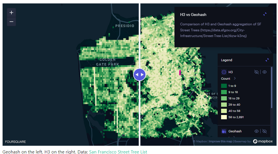
Geohash vs H3: Which Geospatial Indexing System Should I Use?

Geohash vs H3: Which Geospatial Indexing System Should I Use?

For years, the go-to geospatial indexing system has been Geohash. However, a relative new contender has emerged, challenging the status quo – H3. So should you use Geohash or H3?

Here, we’ll explore the differences between Geohash and H3, to help you decide which geospatial indexing system best suits your needs.

Geohash: A Familiar Friend

Geohash is a widely-used geocoding system that encodes geographic coordinates into a short string of letters and numbers. It divides the world into a grid of rectangles, each with a unique Geohash code. The longer the Geohash string, the more precise the location it represents.

H3: The Challenger

H3, on the other hand, is a relatively newer geospatial indexing system that’s gaining traction for its unique approach. Developed by ride-sharing company Uber, H3 uses a hexagonal grid to represent the Earth’s surface. Each hexagon is assigned a unique H3 index, offering a different perspective on geospatial indexing compared to Geohash.

Comparing Geohash and H3

We delve into the main differences between Geohash and H3 on a number of measures.

Precision

  • Geohash: Precision varies based on the length of the code. Longer codes are more precise, but this increases storage and complexity.
  • H3: H3 offers consistent precision regardless of location. Hexagons can be further subdivided for more precision, ensuring uniformity.

Spatial Relationships

  • Geohash: Geohash’s rectangular grid can struggle to represent spatial relationships accurately, especially near the poles (it should be noted that realistically, this is not going to be an issue in most use cases).
  • H3: H3’s hexagonal grid provides better spatial relationships, making it ideal for applications like ride-sharing services and navigation.

Support and Ease of Use

  • Geohash: Geohash is simple and widely adopted, making it easier to find resources and libraries for various programming languages.
  • H3: While H3 is gaining popularity, it may not have the same level of community support and resources as Geohash.

Applications

  • Geohash: Geohash is well-suited for applications that require basic geospatial indexing, such as location-based search or geofencing.
  • H3: H3 shines in complex applications like urban planning, logistics, and ride-sharing due to its consistent precision and better spatial relationships.

Scalability

  • Geohash: As Geohash codes get longer for more precision, storage and indexing can become inefficient.
  • H3: H3 scales more efficiently because it maintains uniform precision, regardless of location.
Geohash vs H3 Comparison

Source: H3

Geohash or H3: Choosing the right system

When it comes down to the choice between Geohash and H3, it really depends on your specific needs:

  • If you require a straightforward geospatial indexing system for basic applications, Geohash is a reliable choice with extensive community support.
  • On the other hand, if you’re dealing with complex spatial relationships, require consistent precision, or are working on innovative projects like urban planning or ride-sharing services, H3 offers a more promising solution. In the real estate context, it can be useful in urban planning, geofencing, spatial analysis, property market analysis.

Geospatial indexing is a fundamental technique used to manage and organise geographic or location-based data efficiently, in order to make data-based decisions or enhance applications.

Geohash is the old guard, tried and tested, while H3 is the newcomer with fresh ideas and uniform precision.

As we can see, both Geohash and H3 have their merits. However, the ultimate decision of which system to use should be based on the requirements of your project.

Snowflake releases H3 functionality

Snowflake provides SQL functions that enable you to use H3 with GEOGRAPHY objects.
This preview feature is now available to all accounts.

Read more blogs from The Proptech Cloud

Australia’s Migration Trends: Where Are People Moving To?

This detailed visual analysis for Australia’s major capital cities breaks down how net migration trends are evolving across different regions.

How to Predict Migration Patterns using Auspost Movers Statistics Data and Snowflake’s Cortex ML functions

How to predict the Australia postcodes people are most likely to relocate to using the Australian Post Movers Statistics dataset and Snowflake Time Series Forecasting function.

Could a Revamp of Australian Property Planning Rules Solve Some of Australia’s Housing Issues?

Rising property prices and high costs of living means the Australian dream of home ownership is slipping further away for many. Could the answer lie in a revamp of property planning rules?

Top Real Estate Technology Global Events

Staying abreast of the latest trends, technologies, and innovations is crucial for professionals seeking to leverage the full potential of real estate technology and proptech.

What Are Mesh Blocks & How Are They Used in Real Estate

What are Mesh Blocks? As defined by Australian Bureau of Statistics (ABS), mesh blocks are the smallest geographical area of the Australian Statistical Geography Standard (ASGS) and ABS’s classification of Australia into a hierarchy of statistical areas. Mesh Blocks...
Geohashes and Efficient Geospatial Joins in Snowflake

Geohashes and Efficient Geospatial Joins in Snowflake

Geohashes are an incredibly useful tool when it comes to spatial analysis. They serve as an encoding system that translates geographic coordinates into a short string of letters and digits, which simplifies and optimises geospatial operations.

One area where geohashes shine is in making geospatial joins more efficient. In this blog, we’ll dive into what geohashes are, and how you can leverage Snowflake’s ST_GEOHASH function to improve your geospatial joins in Snowflake.

What is a geohash?

A geohash is a hierarchical spatial data structure that subdivides space into a grid of cells, each cell having a unique string identifier. Geohashes convert a two-dimensional geographic coordinate (latitude and longitude) into this alphanumeric string. The length of the string determines the precision of the geohash; a longer string means a more precise location.

Read our blog on What is a Geohash for a detailed overview.

Geohash

How geohashes make geospatial joins more efficient

Geospatial joins can be computationally expensive because they often require pairing each record in one dataset with every record in another to calculate distances or find overlaps. This can lead to a computational complexity of O(N*M), which is not ideal for large datasets.

Geohashes simplify this problem by converting the geospatial coordinates into strings. When you want to join based on geographic proximity, you can simply perform a string comparison, which is far less computationally expensive than a full spatial join.

Snowflake and ST_GEOHASH

Snowflake offers native support for geospatial functions, including ST_GEOHASH. Below is a simple example of how you can use this function to create a geohash in Snowflake:

-- Create a geohash for a specific latitude and longitude
SELECT ST_GEOHASH(37.7749, -122.4194, 12) AS geohash;
In this example, 37.7749 is the latitude, -122.4194 is the longitude, and 12 is the precision of the geohash.

To perform a geospatial join using geohashes, you can do the following:

-- Create two tables with geospatial data
CREATE TABLE locations1 (id INT, latitude FLOAT, longitude FLOAT);
CREATE TABLE locations2 (id INT, latitude FLOAT, longitude FLOAT);

-- Populate tables (this is just a representation)
-- ...

-- Add a geohash column to both tables
ALTER TABLE locations1 ADD COLUMN geohash STRING;
ALTER TABLE locations2 ADD COLUMN geohash STRING;

-- Update the geohash columns using ST_GEOHASH
UPDATE locations1 SET geohash = ST_GEOHASH(latitude, longitude, 12);
UPDATE locations2 SET geohash = ST_GEOHASH(latitude, longitude, 12);

-- Perform the join using the geohash
SELECT a.*, b.*
FROM locations1 a, locations2 b
WHERE a.geohash = b.geohash;


Geohash – Streamlining geospatial joins

Geohashes offer a streamlined way to perform geospatial joins, drastically reducing the computational resources required. With native functions like ST_GEOHASH in Snowflake, it’s easier than ever to incorporate geohashes into your geospatial workflows. By leveraging the power of geohashes, you can perform complex geospatial analyses more efficiently, saving both time and money.

Read more blogs from The Proptech Cloud

Australia’s Migration Trends: Where Are People Moving To?

This detailed visual analysis for Australia’s major capital cities breaks down how net migration trends are evolving across different regions.

How to Predict Migration Patterns using Auspost Movers Statistics Data and Snowflake’s Cortex ML functions

How to predict the Australia postcodes people are most likely to relocate to using the Australian Post Movers Statistics dataset and Snowflake Time Series Forecasting function.

Could a Revamp of Australian Property Planning Rules Solve Some of Australia’s Housing Issues?

Rising property prices and high costs of living means the Australian dream of home ownership is slipping further away for many. Could the answer lie in a revamp of property planning rules?

Top Real Estate Technology Global Events

Staying abreast of the latest trends, technologies, and innovations is crucial for professionals seeking to leverage the full potential of real estate technology and proptech.

What Are Mesh Blocks & How Are They Used in Real Estate

What are Mesh Blocks? As defined by Australian Bureau of Statistics (ABS), mesh blocks are the smallest geographical area of the Australian Statistical Geography Standard (ASGS) and ABS’s classification of Australia into a hierarchy of statistical areas. Mesh Blocks...